Basic Principles of Protein X-ray Crystallography
We explore historical aspects of protein X-ray crystallography and explain the basics of the technique and its practical implementation: X-ray data collection, electron density calculations, model building, and refinement.
Protein X-ray Crystallography: Short History
Although, as discussed in the introduction, the technique of protein crystallography was discovered at the beginning of the 20th century, the world had to wait an additional 45 years before the first X-ray crystallographic structure of a protein was determined. This structure was of myoglobin, and earned the authors, Max Perutz and John Kendrew, the Nobel Prize in Chemistry in 1962 “for their studies of the structures of globular proteins”. Since then, many other protein X-ray structures have also received the Nobel Prize. Probably the most spectacular among them was the structure of the ribosome, for which Ada Yonath, Venki Ramakrishnan, and Thomas A. Steitz received the Nobel Prize in Chemistry in 2009.
The structural revolution of the 1990s and around 2000 resulted in an explosion in the number of X-ray structures in the Protein Data Bank. The growth of PDB content has been impressive, with the current number of experimental structures, determined by protein crystallography, NMR spectroscopy, and Cryo-EM, well over 200,000 (see statistics on our structure databases page). The high number of experimental structures paved the way for the creation of AI-based protein structure prediction techniques, the first of which was AlphaFold, an AI system developed by DeepMind to predict protein structures from their amino acid sequence. The latest release of the database includes more than 200 million predicted structures for nearly all proteins cataloged in the scientific literature. This will significantly enhance our understanding of biological processes and elevate structural biology to new levels. This also means that the ability to use and analyze structural information in everyday work in life sciences becomes even more accessible. This work by David Baker (University of Washington), Demis Hassabis, and John Jumper (Google DeepMind) was awarded the Chemistry Nobel Prize in 2024.

Max Perutz and John Kendrew determined the first protein crystallographic structure.
It should be noted that despite this enormous success, the role of experimental structure determination remains very important in many areas of structural biology where more accurate structural details are essential. An example is protein-ligand interactions and the effects of ligand binding on protein conformational dynamics, which is critical in structure-based drug design. Additionally, determining the structure of oligomeric forms and investigating structural dynamics in solution remain areas where experimental data is highly relevant.
How Does Protein X-ray Crystallography Work: Bragg’s Law
X-ray diffraction occurs due to the scattering of electromagnetic waves by the electrons within the crystal lattice. Each electron, when struck by the X-ray beam, acts like a miniature X-ray source. This phenomenon is analogous to a stone thrown into a lake, where the stone serves as the source of the waves. The scattered waves from all the electrons in each atom combine in a process known as interference. In certain directions, the waves will cancel each other out, while in others, they will reinforce and increase in amplitude. This process leads to diffraction, which can be detected by specialized detectors.
If we continue with the analogy of a stone thrown into a lake, to observe interference, we need to throw at least two stones into the water. By watching the waves from the two rocks, we will see that they reinforce or weaken each other. Many interference simulators are available online; an excellent site where you can visually study the effect of wave addition and subtraction (constructive and destructive interference) can be found here. More options can be found on the PhET simulation site; they even have some videos on YouTube with a demonstration of the simulations. For this reason, I don’t show any examples here.
As discussed in the introduction, the Braggs were the first to propose a physical model for describing X-ray diffraction. In Bragg’s model of diffraction, the crystal lattice is viewed as a series of atomic layers that, like a mirror, reflect the X-rays striking the crystal. When the path difference between waves reflected from the layers is an integer multiple of the X-ray wavelength, the reflected waves are in phase and combine constructively, becoming stronger. If the path difference is not an integer multiple of the reflected X-rays, they will be out of phase and cancel each other out. Mathematically, Bragg’s law looks like this: nλ = 2d sinθ, where n is an integer, d is the interplanar distance in the crystal, and θ is the incident angle of the X-rays. We can immediately see from this expression that by changing the θ angle, we bring different planes of the crystal into the position of constructive interference. This is also used in X-ray crystallography: the crystal is mounted on a device called a goniometer, which can be rotated in the X-ray beam to collect data from all possible lattice planes of the crystal.
X-ray Data Collection
X-rays may be generated using laboratory X-ray sources or at synchrotrons, where very high intensity and highly focused X-rays can be generated. Several synchrotrons worldwide have stations adapted for collecting X-ray data from protein crystals. In Lund, we use the BioMax beamline at the MAX IV synchrotron. Depending on the type of crystal (crystals may have different cell dimensions and symmetry groups), different strategies for data collection are followed. As mentioned above, in a standard setup, the crystal is rotated in the X-ray beam one degree or less at a time and exposed to X-rays for a short period (seconds or less) until a complete data set is collected. The total data collection time depends on the intensity of the X-ray source, the size of the crystal, how well it diffracts (resolution), and the symmetry of the crystal. The data are subsequently processed using dedicated software (a process in crystallography called “data reduction”). Several software packages serve this purpose.
When collecting data in X-ray crystallography, it is crucial to prioritize data quality. Even while overlooking the experimenter’s errors and assuming that data collection is conducted at a high professional standard, the data quality still hinges on the crystals used. Some crystals may yield high-quality data, while others may diffract poorly. If we find that the diffraction is subpar (low solution, diffraction spots appear blurry, presence of twinning, ice rings, etc.), we can attempt to enhance the crystal quality. In certain instances, this approach may be practical, but at times, improving the crystal quality can prove challenging. Poor data quality may result in poor electron density, which in turn will affect the quality of the final protein structure built into this density. This needs to be taken into account when validating the quality of the structure.
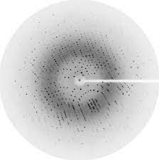
Generally, resolution is the primary factor determining the quality of the data and the protein structure. High resolution guarantees better structure. The resolution for a given crystal (a specific crystal lattice and type of symmetry) is roughly determined by the number of diffraction spots (intensities) collected during a crystallography experiment. Each spot contains information from a distinct Bragg plane, and the higher the number of spots we collect, the more data we get from different Bragg planes, which gives us more detailed information to calculate the electron density map and build the structure. The diffraction images on the right for a well-diffracting crystal (many spots going to the edge of the image) and a crystal diffracting at low resolution (few spots around the center) illustrate this principle.
What is a good resolution?
Below are some approximate ranges of resolution to be able to put the numbers on some relative scale:
Low resolution – in the range from extremely low to low, up to 5 Å. Here, the overall shape of the molecule is distinguishable; at around 5 Å, we can see helices as long rods, but no detailed model building is possible.
At medium resolution (3.5-2.5 Å), we start to distinguish side chains and build the model. When the resolution is better than 2.8 Å, we start to see some water density and can build some water molecules into the density.
Atomic resolution (2.4 Å and better): The model-building process starts to be a pleasure; solvent molecules can be easily identified.
Electron Density Calculation
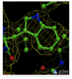
On a diffraction image, which is obtained during data collection, each spot corresponds to an X-ray beam from a particular set of Bragg planes, as described above. Thousands of such spots from all possible lattice planes must be collected from a protein crystal to get a complete data set. The relative intensities of the spots are extracted during data processing and used to calculate the structure factors F(hkl) and an electron density map of the molecules inside the crystal. The electron density, in turn, will tell us where the atoms are located, information that is used to build a model of the molecule. The image on the right shows a triptophan side chain built into its electron density.
For the calculation of the electron density, we need to re-integrate the collected “waves” in a mathematical operation called the Fourier summation.
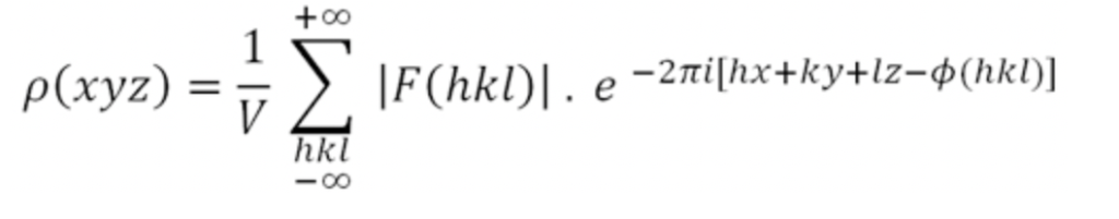
In the equation, the structure factor F(hkl) is derived from the diffraction image using the intensities of the diffraction spots. It represents the diffracted beams from all atoms within the Bragg planes mentioned earlier. In practical applications, crystallography works with a so-called unit cell (see below). h, k, l are referred to as the Miller indices of the diffracted beams. Each Bragg plane is assigned a Miller index, which describes the location of the diffracted spot in what is called the reciprocal space. Φ(hkl) denotes the phases of the diffracted wave, and V indicates the volume of the unit cell.
As we can see from the equation, for this operation to work, the phase Φ(hkl) of each diffracted beam is essential. The phase is lost during data collection and must be determined using alternative methods. One such method, heavy atom replacement, was quite popular in the early days of protein crystallography.
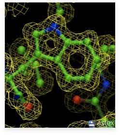
The upper image shows the model of the tryptophan side chain inside its high resolution electron density (1.15 Å, alcohol dehydrogenase, PDB ID 1HET). The image below shows the same side chain with the electron density at 3 Å resolution (Donkey hemoglobin, PDB ID 1SOH). Clearly, the positions of the atoms at high resolution are defined with considerably higher accuracy.
However, currently, other, more efficient methods that utilize the tunability of the X-ray beam wavelength at synchrotrons are in use. Additionally, the method of molecular replacement is frequently employed. Molecular replacement uses the known structure of a homologous molecule to calculate the initial set of phases. With the advent of the AlphaFold structure prediction, predicted structures can sometimes also be used for initial phasing.
Refinement and the R-factor
In protein crystallography, after building a structural model, it is subjected to several cycles of refinement and model building (model adjustments). The quality of the electron density map used in model building depends on the resolution of the X-ray data and on the quality of the phases used in the density calculations. The better the map quality, the easier it will be to refine the model. During several refinement cycles, the initial structural model is adjusted to fit the electron density as accurately as possible. A parameter called the R-factor is calculated to assess the accuracy of the model fit to the experimental data. Below is the equation used to calculate the R-factor:
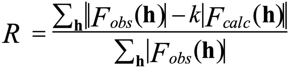
In this equation, F_obs and F_calc represent observed and calculated structure factors. The structure factor F_obs is derived from the measured diffraction intensities, while F_calc can be calculated from the model structure built into the electron density using the Fourier transformation. Intuitively, we can see from the equation that the closer F_obs and F_calc are, the lower the R-factor will be. The R-factor is an essential parameter in the assessment of model quality. A lower R-factor shows that the model is a better fit for the experimental data. For protein crystals, the R-factor for refined structures typically ranges from 25% to 14%, whereas for small molecule structures, it is usually around 4%. Additional discussion on the use of the R-factor can be found in the section on model validation and quality assessment.
Crystal Symmetry and the Asymmetric Unit
We also need to remember that PDB files contain the so-called asymmetric unit of the crystal. The functional biological unit (the quaternary structure) in solution may contain several subunits of the same protein, arranged as dimers, trimers, or larger-order oligomers. Often, the subunits in these quaternary structures in solution are related by some symmetry, for example, two-, three-, or four-fold rotation. When crystallized, the oligomer symmetry axis may become a crystallographic symmetry axis. This means that a monomer within a dimer, a trimer, or a tetramer becomes an asymmetric unit of the crystal.
Why is it an asymmetric unit and a crystallographic symmetry axis? When the molecules are crystallized, they are arranged in the space lattices of the crystal. Within this lattice, all molecules are ordered and related to each other by crystallographic symmetry operations of the symmetry group of that crystal (the possible symmetry groups are listed in a book called International Tables for Crystallography). A symmetry operation represents a mathematical transformation that, when applied to the coordinates of one molecule, will transform it to its symmetry-related mate in the crystal lattice. This is what we mean when we say that molecules in the crystal lattice are arranged according to certain symmetry operations. By applying symmetry transformation to the asymmetric unit, we can generate all other molecules in the crystal. For example, a trimer may be easily generated by applying the mathematical operations of the 3-fold rotation axis. For this reason, calculations in crystallography are performed using only the asymmetric unit of the crystal. All related molecules in the crystal are assumed to be precisely similar.
This is reflected in the content of the PDB files, which only contain the atomic coordinates of the asymmetric unit. However, the PDB server reconstructs the biological unit when it is known to be different from the asymmetric unit. If we need the biological unit, we may choose it when viewing the 3D structure in the graphics display or when downloading the coordinate file.
For clarity, the concept of the asymmetric unit is illustrated in the image below:
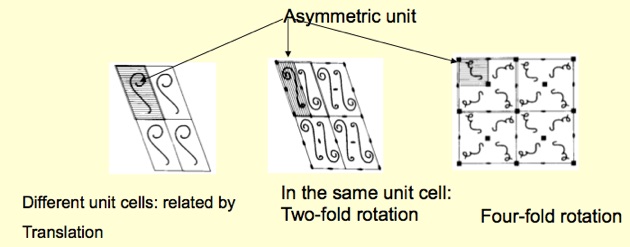
The asymmetric unit of a crystal
In the left figure, the asymmetric unit of a crystal, which represents just “one subunit”, is shown. All molecules in the lattice are related to one another by simple translation. In the example in the middle, two subunits in the unit cell are related by a two-fold rotation axis (180 degrees of rotation). This suggests that the protein in the solution (the biological unit) may be a dimer. The third example on the right illustrates that a 4-fold crystallographic symmetry relates the molecules in the unit cell. Again, this indicates that the biological unit in solution is a tetramer. In all these cases, the asymmetric unit is a monomer, but we may also encounter a dimer, trimer, etc., in the asymmetric unit. In this case, the rotation operations will be applied to the respective dimer or trimer, producing, e.g., a trimer of dimers, a tetramer of trimers, etc. Additional experiments like dynamic light scattering (DLS) or small-angle X-ray scattering (SAXS) may be needed to verify the protein’s oligomeric status in the solution.